South Pole Telescope low-\(\ell\)

This plugin implements the South Pole Telescope likelihood from Story et al. (2012) and Keisler et al. (2011). The data comes included with this plugin and was downloaded from here and here, respectively.

You can choose which likelihood to use by specifying which='s12' or which='k11' when you initialize the plugin.

The plugin also supports specifying an \(\ell_{\rm min}\), \(\ell_{\rm max}\), or dropping certain data bins.

%pylab inline

Populating the interactive namespace from numpy and matplotlib

from cosmoslik import *

Basic Script

Here’s a script which runs a basic SPT-only chain:

class spt(SlikPlugin):

    def __init__(self, **kwargs):
        super().__init__()
        self.cosmo = models.cosmology("lcdm")
        self.spt_lowl = likelihoods.spt_lowl(**kwargs)
        self.cmb = models.camb(lmax=4000)
        self.sampler = samplers.metropolis_hastings(self)

    def __call__(self):
        return self.spt_lowl(self.cmb(**self.cosmo))

Four sampled parameters, one for calibration and three for foregrounds, come by default with the SPT plugin:

spt().spt_lowl.find_sampled().keys()

odict_keys(['cal', 'egfs.Acl', 'egfs.Aps', 'egfs.Asz'])

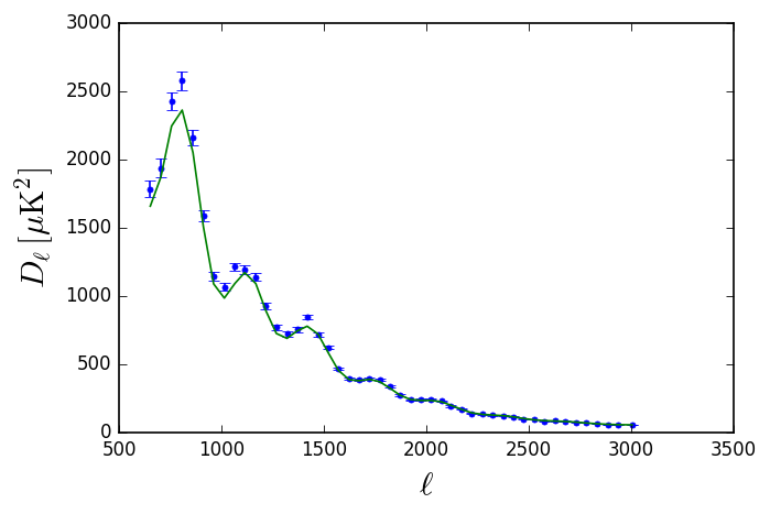
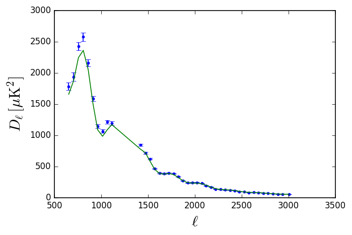
The plugin has a convenience method for plotting the data and current model:

s = Slik(spt(which='s12'))
lnl, e = s.evaluate(**s.get_start())
e.spt_lowl.plot()

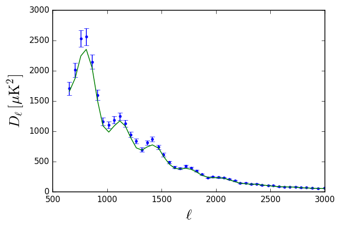
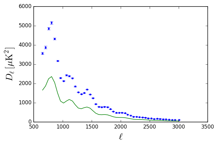
Or you can plot the “k11” bandpowers. You can see they’re less constraining.

s = Slik(spt(which='k11'))
lnl, e = s.evaluate(**s.get_start())
e.spt_lowl.plot()

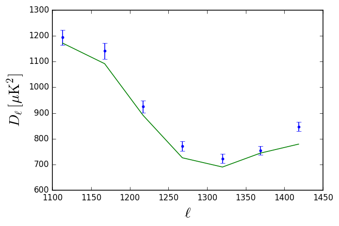
Choosing subsets of data

You can also set some \(\ell\)-limits,

s = Slik(spt(which='s12',lmin=1000,lmax=1500))
lnl, e = s.evaluate(**s.get_start())
e.spt_lowl.plot()

Or drop some individual data points (by bin index),

s = Slik(spt(which='s12',drop=range(10,15)))
lnl, e = s.evaluate(**s.get_start())
e.spt_lowl.plot()

Calibration parameter

The calibration parameter is called cal and defined so it multiplies the data bandpowers. For “s12” it comes by default with a prior \(1 \pm 0.026\). You can’t use it for “k11” because this likelihood has the calibration pre-folded into the covariance.

s = Slik(spt(which='s12',cal=2))
lnl, e = s.evaluate(**s.get_start())
e.spt_lowl.plot()

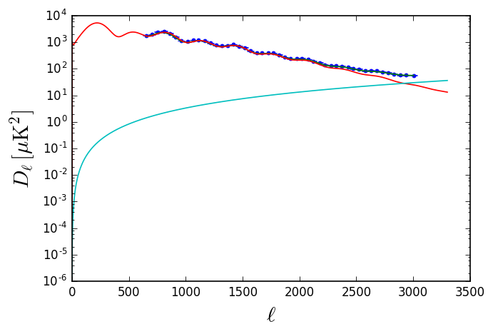
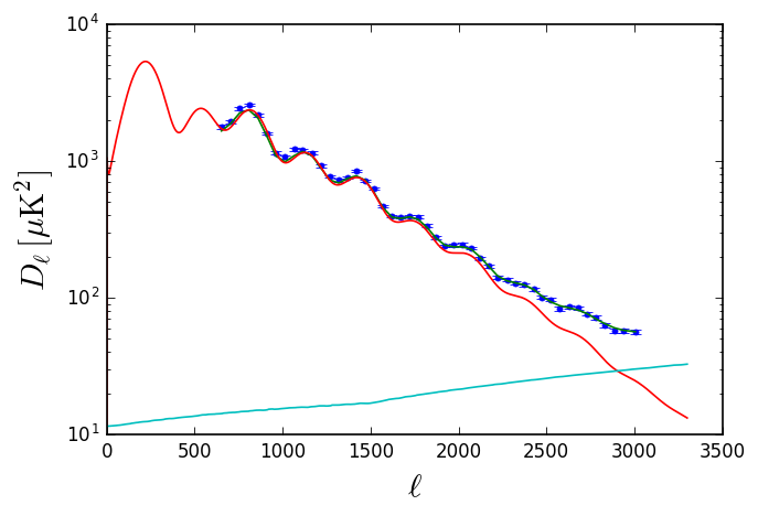
Foreground model

By default the foreground model is the one used in the Story/Keisler et al. papers (same for both). There’s an option to plot which shows you the CMB and foreground components separately so you can see it.

s = Slik(spt(which='s12'))
lnl, e = s.evaluate(**s.get_start())
e.spt_lowl.plot(show_comps=True)
yscale('log')

The foreground model is taken from the spt_lowl.egfs attribute which is expected to be a function which can be called with parameters lmax to specify the length of the array returned, and egfs_specs which provides some info about frequencies/fluxcut of the SPT bandpowers for more advanced foreground models. You can customize this by attaching your own callable function to spt_lowl.egfs when you call __init__, or passing something in during __call__.

For example, say we wanted a Poisson-only foreground model, we could write the script like so:

class spt_myfgs(SlikPlugin):

    def __init__(self):
        super().__init__()
        self.cosmo = models.cosmology("lcdm")
        self.spt_lowl = likelihoods.spt_lowl(egfs=None) #turn off default model & params
        self.Aps = param(start=30, scale=10, min=0) #add our own sampled parameter here
        self.cmb = models.camb(lmax=4000)
        self.sampler = samplers.metropolis_hastings(self)

    def __call__(self):
        return self.spt_lowl(self.cmb(**self.cosmo),
                            egfs=lambda lmax,**_: self.Aps * (arange(lmax)/3000.)**2) #compute our foregroud model

s = Slik(spt_myfgs())
lnl, e = s.evaluate(**s.get_start())
e.spt_lowl.plot(show_comps=True)
yscale("log")